
Portfolio Allocation
Portfolio Allocation problems revolve around dividing the capital you have into a set of assets such that the risk is minimized and the returns are maximized. It involves assigning a weight to each investment. For example, if we’re investing £1.000 in 5 stocks, we need to divide that money into 5 parts for each stock. Deciding how much money goes into each stock is at the hart of portfolio allocation.
An obvious distribution would be to give £200 equally for each stock. But since we have more information about the stock (volatility, expected returns, etc), we can use this information to have a better distribution of capital.
In this guide, I’m going to be using risk as a method of distribution. A simple risk model is that risk is associated with the variance of a stock. A stock with more variance is riskier than the one with less variance.
Context For The Marcenko-Pastur theorem
A common way to evaluate risk of a group of stocks is to find their covariances matrix. Then using principal component analysis, we can get a number of possible portfolios and their associated variance. If you don’t know how PCA works, check out my guide for it: PCA from fundamentals.
The problem is that financial data has low signal-to-noise ratio. Which means most of what we get is garbage. How do we figure out what is garbage and what is not? The Marcenko-Pastur distribution helps us.
Given a covariance matrix for a set of stocks, we calculate the set of eigenvalues and eigenvectors for it using PCA. The eigenvectors refer to the weights of each stock that goes into making the principle component and the eigenvalues are the variances of those principle components. Each principle component is a portfolio. The problem is that most eigenvalues we get are variances for the noise of the prices. We use the Marcenko-Pastur distribution to filter out noisy eigenvalues.
The Marcenko-Pastur Theorem
Given a matrix of size TxN , where T is the number of assets and N is the size of data we have for each asset. It is assumed that the entries are all iid with N(0, σ²). So, the entire matrix is composed of noise. The marcenko-pastur theorem provides a distribution of the eigenvalues of this matrix.
Lower and upper bounds of the support of the distribution
Given the size of the matrix T x N , we calculate the “aspect ratio”

Using this and the variance, we calculate the lower and upper bounds of the distribution:

These bounds refer to the minimum and maximum values the eigenvalues can take if the process generating the matrix was entirely random. This is the key point behind the theorem. Any eigenvalue outside this range is signal and any eigenvalue inside the range is noise.
PDF of the distribution
The PDF of the Marcenko-Pastur distribution is provided by:

Testing out the distribution
Before using the distribution, it is good to see how the distribution works. We’ll try two tests. First we’ll have a completely random matrix. All the eigenvalues of this matrix must be within the lower bounds. Then we’ll have a signal matrix with some noise. The theorem should distinguish between the signal and the noise.
Pure Random Matrix
importing the libraries we need:
import numpy as np
import matplotlib.pyplot as plt
import pandas as pd
from sklearn.neighbors._kde import KernelDensity
Getting the random matrix
sigma = 2 # Variance of the entire distribution
x = np.random.normal(size=(10000, 1000), scale=sigma) # A random 10000 x 1000 matrix
Plotting the distribution
q = float(10000 / 1000) # Aspect ratio

# Lower and upper limits
lower_limit = sigma**2 * (1 - np.sqrt(1.0 / q)) ** 2
upper_limit = sigma**2 * (1 + np.sqrt(1.0 / q)) ** 2

# Getting the x-values
lambda_values = np.linspace(lower_limit, upper_limit, 1000)

# Getting the y-values
pdf = q / (2 * np.pi * sigma * lambda_values) * np.sqrt(((upper_limit - lambda_values) * (lambda_values - lower_limit)))
pdf = pd.Series(pdf, index=eVal)

# Plotting the graph
plt.plot(pdf.index, pdf.values)
plt.title("Marcenko-Pastur Distribution")
plt.axvline(x=lower_limit, color="r", linestyle="--", label="Lambda Minus")
plt.axvline(x=upper_limit, color="g", linestyle="--", label="Lambda Plus")
plt.legend()
plt.grid(True)
plt.show()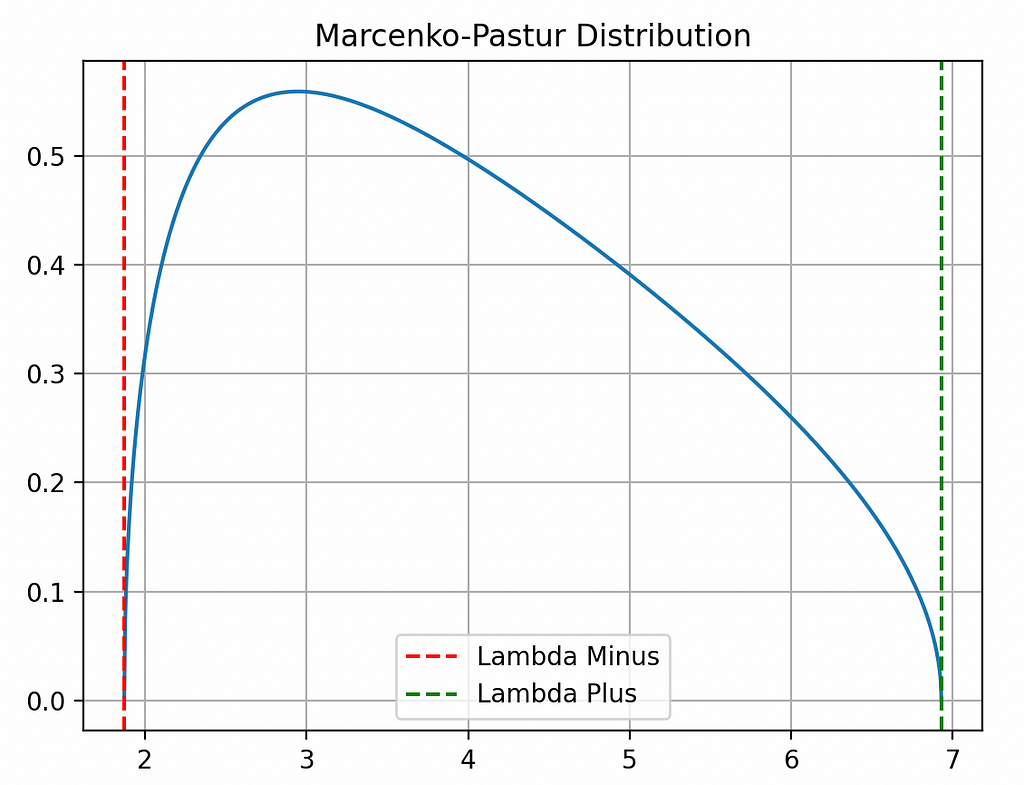
Getting the eigenvalues of the correlation matrix
# Getting the eigenvalues and eigenvectors using the hermitian matrix
eVal, eVec = np.linalg.eigh(np.cov(x, rowvar=0))

# Sorting the eigenvalues and eigenvectors in decending order
indices = eVal.argsort()[::-1]
eVal, eVec = eVal[indices], eVec[:, indices]
Density plot of eigenvalues
We’ll use the Kernel Density Plot to get an approximate distribution of the eigenvalues of the covariance matrix
kde = KernelDensity(kernel="gaussian", bandwidth=0.01).fit(eVal.reshape(-1, 1))
x = np.unique(eVal).reshape(-1, 1)
logProb = kde.score_samples(x)
kde_pdf = pd.Series(np.exp(logProb), index=x.flatten())
Comparing the distributions
plt.figure(figsize=(10, 6))
plt.plot(pdf.index, pdf.values, label="Marcenko-Pastur PDF")
plt.plot(kde_pdf.index, kde_pdf.values, label="Empirical PDF")
plt.axvline(x=lower_limit, color="r", linestyle="--", label="Lambda Minus")
plt.axvline(x=upper_limit, color="g", linestyle="--", label="Lambda Plus")
plt.title("PDF Comparison")
plt.xlabel("Eigenvalue")
plt.ylabel("Density")
plt.legend()
plt.grid(True)
plt.show()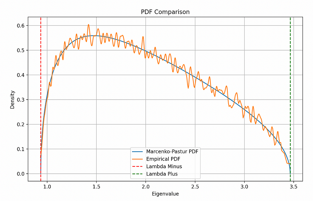
Both the distributions match very well. That’s a good sign.
Semi-random Matrix
Creating a covariance matrix with some structure
def structured_cov_matrix(nCols, nFacts):
    w = np.random.normal(size=(nCols, nFacts))
    cov = np.dot(w, w.T)

    # Ensure full-rank
    cov += np.diag(np.random.uniform(size=nCols))
    return cov
Even though the underlying matrix is random, using the dot product creates some structure, in the sense that each entry in the cov matrix isn’t completely independent. Finally adding the diagonal matrix ensures full-rank.
Noise + Signal matrix
alpha = 0.0095 # Mixing ratio
nCols = 1000 # Number of features
nFacts = 100 # Number of latent factors

# Random noise covariance matrix
cov = np.cov(np.random.normal(size=(nCols * q, nCols)), rowvar=0)

# Adding some signal
cov = alpha * cov + (1 - alpha) * structured_cov_matrix(nCols, nFact)

eVal, eVec = np.linalg.eigh(cov)
indices = eVal.argsort()[::-1]
eVal, eVec = eVal[indices], eVec[:, indices]
Plotting the distribution
Now that we have the covariance matrix, we can get its eigenvalue just like before and plot the histogram of the eigenvalues along with the theoretical distribution
plt.figure(figsize=(10, 6))
plt.plot(pdf.index, pdf.values, label="Marcenko-Pastur PDF")
plt.hist(eVal, density=True, bins=50, label="Empirical PDF")
plt.axvline(x=lower_limit, color="r", linestyle="--", label="Lambda Minus")
plt.axvline(x=upper_limit, color="g", linestyle="--", label="Lambda Plus")
plt.title("PDF Comparison")
plt.xlabel("Eigenvalue")
plt.ylabel("Density")
plt.legend()
plt.grid(True)
plt.show()
Notice how most of the eigenvalues lie within the bounds. They represent random noise. But the eigenvalues outside the bounds represent the signal we had added.
Distinguishing between noise and signal
Distinguishing between noise and signal is quite simple. You just have to calculate the lower and upper bounds of the support of the distribution and then check for values outside the range
significant_eigenvalues = [
     ev for ev in eigvals if ev > lambda_plus or ev < lambda_minus
]
Sample use: Portfolio Allocation
Suppose I have a list of 48 stocks I want to trade:
stocks = ["AAPL", "MSFT", "AMZN", "GOOGL", "TSLA", "JNJ", "V", "WMT",
             "PG", "JPM", "UNH", "NVDA", "HD", "DIS", "PYPL", "MA", "NFLX",
             "ADBE", "INTC", "CMCSA", "PFE", "VZ", "KO", "PEP", "MRK", "ABT",
             "NKE", "XOM", "T", "CSCO", "BA", "WFC", "MCD", "CRM", "COST",
             "ACN", "CVX", "MDT", "AVGO", "TXN", "HON", "NEE", "SBUX", "UNP",
             "QCOM", "IBM", "ORCL", "LIN"]
But I don’t know how much capital to put in each one.
I can use historical returns to get my covariance/correlation matrix and used the analysis in this guide to figure out the right portfolio.
Getting stock data:
# Fetching stock data
def fetch_stock_data(stock):
    stock_file_path = f"data/{stock}.csv"
    if not os.path.exists(stock_file_path):
        print(f"File not found for {stock}. Downloading stock data...")
        data = yf.download(stock)
        data.to_csv(stock_file_path)

# Combining all stock data into a single dataframe
combined_df = pd.DataFrame()
for stock in stocks:
    fetch_stock_data(stock)
    stock_ts = pd.read_csv(f"data/{stock}.csv")
    stock_ts.set_index(stock_ts["Date"], inplace=True)
    combined_df[stock] = stock_ts["Close"]

combined_df.dropna(inplace=True)
Calculating the correlation matrix
In this case, I’ll be using the correlation matrix since I don’t know the variance of the underlying process. The variance of MP-distribution for a correlation matrix is just 1.
The correlation matrix is calculated by using the daily returns as a percentage change.
corr_matrix = combined_df.pct_change().dropna().corr()Getting the eigenvalues and eigenvectors
eigvals, eigvectors = np.linalg.eigh(corr_matrix)

eigpairs = [(eigvals[i], eigvectors[i]) for i in range(len(eigvals))]
eigpairs.sort(key=lambda x: x[0], reverse=True)
eigvals = [_[0] for _ in eigpairs]
The Marcenko-Pastur Limits
N = len(corr_matrix)  # Number of assets
T = combined_df.shape[0]  # Number of observations
q = T / N  # Aspect ratio
sigma = 1

lambda_minus = sigma**2 * (1 - np.sqrt(1.0 / q)) ** 2
lambda_plus = sigma**2 * (1 + np.sqrt(1.0 / q)) ** 2
Plotting the eigenvalues with the limits
lambdas = np.linspace(lambda_minus, lambda_plus, 1000)

plt.figure(figsize=(10, 6))
plt.hist(eigvals, bins=50, density=True, alpha=0.5, label="Eigenvalues")
plt.axvline(x=lambda_minus, color="r", linestyle="--", label="Lambda Minus")
plt.axvline(x=lambda_plus, color="g", linestyle="--", label="Lambda Plus")
plt.title("Eigenvalues vs Marcenko-Pastur Distribution")
plt.xlabel("Eigenvalue")
plt.ylabel("Density")
plt.legend()
plt.grid(True)
plt.show()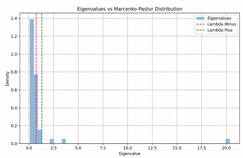
Most of the eigenvalues are insignificant, but there are 3 that are above the upper limit. These are our portfolios of interest.
One of them has a massive eigenvalue of 20. This means it is very risky. The other two seem normal.
Getting the portfolios
portfolios = [pair for pair in eigpairs if pair[0] > lambda_plus]for i in range(len(portfolios)):
print(f"PORTFOLIO {i+1}: ")
print("Variance: ", portfolios[i][0])
print("Weights: ")
print(portfolios[i][1])
print("-----------------------------------------------")PORTFOLIO 1:
Variance: 20.33971657547852
Weights:
[-0.00253896 0.01857771 0.0736624 0.03144459 -0.05088898 0.13688758
-0.09181728 -0.01051777 -0.05160817 0.12208625 0.06683743 0.1999884
-0.09907906 -0.13264177 -0.22091254 0.02013253 0.17973713 -0.13257361
0.04139994 0.22510826 -0.04473338 0.02003644 -0.06063211 0.49788887
0.06450855 -0.44238874 0.01099729 -0.11303053 0.01793605 -0.14393446
0.08309327 0.31361412 -0.15380875 -0.07052455 0.07925522 0.12190625
0.0783257 -0.08384648 0.00605482 -0.01045911 0.05219613 -0.10361418
-0.11880203 0.00943192 0.07847018 0.06018686 -0.05354198 0.16129682]
-----------------------------------------------
PORTFOLIO 2:
Variance: 3.447080645190461
Weights:
[-0.01339223 0.00418134 0.00588765 0.0698238 0.0015164 0.03670837
-0.05065868 0.12866772 0.0266015 -0.06435319 0.08931394 0.06325342
-0.12152671 0.0272931 0.08631622 0.04433468 0.0196137 0.05175692
0.03151782 0.013989 -0.04423597 -0.2547019 0.19854827 0.01569395
0.14504711 0.04084806 0.2085682 -0.12915807 0.50946264 -0.03595187
0.00337607 -0.16695716 0.09533894 -0.24557398 0.01921367 -0.12740803
0.10974681 0.07138481 -0.36149868 0.14301944 0.37678964 0.00892604
-0.01966316 0.16900382 -0.03502878 -0.05006935 0.03768993 0.14094934]
-----------------------------------------------
PORTFOLIO 3:
Variance: 2.2094175455188996
Weights:
[ 0.01737647 0.02744565 -0.01202147 -0.04720913 -0.00443812 -0.0296574
0.01045607 0.0176474 -0.02154059 0.22284979 0.00709835 -0.0343424
-0.17190634 0.07311515 -0.17019518 0.0341493 -0.11300356 -0.07261734
-0.12952617 -0.01701636 0.01575385 0.07419057 0.28173015 -0.19717795
0.17104962 -0.22886315 -0.48659551 0.08176375 -0.30173463 0.04011432
-0.2168248 -0.08761059 0.12596135 -0.06708469 -0.1742353 0.1118194
-0.00617398 -0.00129855 -0.2197061 0.12831287 0.18585968 -0.09824587
-0.01066517 0.18386141 -0.06638463 0.0537813 -0.11098294 0.14690054]
-----------------------------------------------Conclusion
The Marcenko-Pastur theorem is a powerful tool for filtering noise from financial data, allowing for more effective portfolio allocation. By distinguishing between eigenvalues that represent meaningful signals and those that represent noise, we can identify the principal components that truly impact our portfolio’s risk and return.